Automated Threat Hunting for Network Beacons Using Zeek and Math
Understanding Command and Control (C2) Malware
Generally speaking, most people associate typical “computer hacking” with the idea of being able to remotely control a computer system without the consent of the computer system’s owner. It can be considered the holy grail of any engagement performed by red teams or advanced persistent threats (APTs), as you need to compromise some system on an organization’s network before further attacks against the organization can occur. Red teamers and advanced persistent threats (APTs), which will be referred to as adversaries for the rest of this blog post, tend to do this in one of two ways:
Social engineering an employee to execute malware that allows the adversary to control the employee’s system
Exploiting a publicly facing website or service by having it execute malware that allows the adversary to control the publicly facing website or service
The second method does not occur often due to the amount of security controls that tend to exist on publicly facing sites and services, so the first method is way more practical as it’s always much easier to hack a person than it is a computer system. Regardless of the means of how adversaries gain control of the systems, the malware that allows adversaries to remotely control a computer system is known as command and control (C2) malware:
C2 malware works by periodically connecting back to an adversary-controlled server. Through the adversary-controlled server, the adversary can issue commands to the malware for it to execute on the compromised computer system, allowing the adversary to remotely control the compromised system and perform various actions on it. The functionality of C2 malware is quite advanced and can perform actions like reading files, exfiltrating data, or even reaching out to other systems on the same network as the compromised computer system in order to establish C2 on those computer systems as well. For cybersecurity professionals, the presence of C2 malware in an environment is bad news.
How Beaconing Works
In order for C2 malware to work, it needs to connect back to the adversary-controlled server so it can receive commands to execute on the compromised system. This “connect back” process utilizes a network connection that typically acts in one of two ways:
The connect back is a long lived connection that stays alive for as long is needed
The connect back happens on some regular cadence
The second option is what we’ll be taking a look at today, the act of which is known as beaconing. Beaconing is the process of C2 malware initiating network connections to adversary-controlled servers on some regular interval. The interval is completely controlled by the adversary, and tradeoffs exist depending on how frequently the C2 malware beacons. If the adversary wants faster responses from the C2 malware and being covert doesn’t matter too much (like during a penetration testing engagement), then they may have a high frequency beacon that occurs every 1-5 seconds. If the adversary wants to stay a little more covert and blend with the network, then they may have a lower frequency beacon that occurs once an hour, couple of hours, or even longer.
As you can probably already deduce, higher frequency beacons come with more risk due to larger amounts of network activity. If a network connection is regularly occurring, then there’s a higher likelihood that it’ll be detected. In an attempt to combat this, adversaries can what’s known add a “jitter” to the frequency which varies the timing of the beacons. Instead of a beacon occurring every 60 seconds exactly, adversaries can add a 10 second jitter so that the beacon can occur every 50 - 70 seconds, making the network connection much less routine in nature.
How to Threat Hunt for Beacons
Beacons by definition are regularly occurring network connections regardless of their intervals. This means that if you look at how much time passes between each beacon connection, it will be relatively the same. For example, if you take five random samples of a beacon initiating network connections that occur every 60 seconds with a 5 second jitter, then you can have a beacon with times between connections that looks like the following:
[60, 56, 63, 59, 64]
In this example, you can see that the timing between each beacon connection is relatively small even if the difference between each beacon isn’t exactly uniform. In other words, the dispersion between the times is relatively small. Network connections initiated by people are much less routine in nature. Therefore, if there is a way to measure how big the dispersion is between connections, you’ll have a way to determine beacons in your environment. Measuring the dispersion is where the mathematical concept of standard deviation comes into play. Standard deviation is defined as “a measure of the amount of variation of a random variable expected about its mean”. In other words, the above example, the mean for the first 5 connections is 60.4, and the standard deviation is 2.871. If you take a similar example of a beacon initiating network connections that occur every 60 seconds without jitter, then you’ll have a beacon with the following times:
[60, 60, 60, 60, 60]
For this sample, the mean of the times in between connections is 60 and the standard deviation between the times is 0. Therefore, we know that the times between beacons tend to have lower standard deviations. Putting all this knowledge together, we can use the following steps to hunt for beacons:
Gather network logs over a given timeframe (e.g. 30 days)
Determine the source/destination pairs for network connections in the network logs, making sure to only note the network connections that initiate connections outside of the network
Calculate the timing between each unique source/destination network connections as a list
Determine the standard deviation for each unique source/destination list
Collect the standard deviations that fall in the lowest percentile (e.g. the standard deviations that fall within the lowest 5% of values)
However, this approach does have its downfalls:
You need to collect network logs over a long enough timeframe, as some beacons have longer intervals that may not show up over short periods
Higher jitter values makes detection more difficult, as it makes the beacon interval more random
Legitimate automated network activity (such as system monitors) will show up in the results, although this may not be too bad of a hurdle as it’s easy to find the public IPs of official service providers like Microsoft, Google, etc.
Finding beacons with higher jitter will require baselining your network which can be done with deep learning methods, but is outside of the scope of this post.
To see an application of this methodology, let’s apply it to an example threat hunt provided by Active Countermeasures.
Threat Hunting for Beacons in Zeek Logs
The threat hunting challenge provided by Active Countermeasure involves the AsyncRAT malware that beacons every 6.5 seconds with a 1.5 second jitter. The malware has been executed on a system within a lab environment. Logs have been collected over 24 hours within the lab environment, meaning that you’re getting network logs of all the systems in the lab environment and not just the compromised system. These logs can be found here.
The first step has already been completed in terms of collecting the logs, which consist of 24 hours of network logs found in the conn.log file.
The second step will be determining the source/destination pairs for network connections from the logs. This can be performed with some Python scripting as shown below, which reads logs and determines the unique source/destination pairs of the network:

Reading Zeek logs and parsing unique source/destination pairs
The third step involves calculating the timings between each source/destination pair. For each pair, the script will find all lines involving these sources/destinations and log the times associated with the connections, making sure to exclude any destinations that involve the local network. The script then calculates the timing between each of the network connections as shown below:

Determining the times of each connection and calculating the timing in between connections
The fourth step involves calculating the standard deviation for the list of differences for each source/destination pair. This is performed using the standard deviation function provided by the numpy library, as seen below:
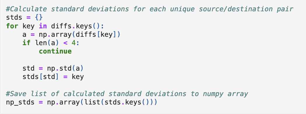
Calculating standard deviations between connections
The last step is finding the standard deviations that are considered low relative to the other standard deviations for the other connections. This is performed using the percentile function provided by the numpy library. Using the right percentile involves a little experimentation, but this example uses the 5th percentile, meaning that we’re concerned with all standard deviations from network connections that fall at the 5th percentile or lower, as shown below:

Finding the low standard deviations as well as the number of connections for the low standard deviations
You’ll notice that two source/destination pairs appear, with the destinations being 184.150.58.155 and 172.208.51.75. With a beacon timing of 6.5 seconds with a 1.5 second jitter, you can assume that a lot of connections will happen over the 24 hours of the logs. You can figure out which of these has more network connections by going back to the timings processed in the third step of this process. The number of connections to 184.150.58.155 is 5, while the number of connections to 172.208.51.75 is 13,281. This is definitely anomalous relative to the number of other outbound connections in the logs, and it turns out that this is the malicious IP address where the AsyncRAT malware beacons.
The actual threat hunt provides more information in order to reach this conclusion (which you should read), but this post is more to show how beaconing can be found in network logs in an automated fashion.
Conclusion
This was a great example of how basis statistics can be used to automate threat hunting in your environment. For actual hunts, there may be more network connections to account for as well as the filtering of known good IP addresses (e.g. Microsoft IP addresses, Google IP addresses, Akamai IP addresses, etc). It may even help to baseline the network for anomalous connections via deep learning methods, which we hope to cover in a future post. However, the methodology of finding beacons remains the same and hopefully you can use it in your own threat hunting practice. The code used in this post can be found on the official QFunction GitHub here. If you’re interested in automated threat hunting, check out how QFunction performs AI-based threat hunting! And if you’re interested in another Zeek network threat hunt using deep learning methods, check out our post on threat hunting Zeek logs using AI!